In our last post on this topic we left off asking the question, “given how much wildland fires change year to year, how do we build an emissions inventory (EI) that is representative of a multi-year period, or a future period?” This is a confounding problem not only for the Regional Haze planning process but for any air quality planning exercise that a regulatory agency engages with.
In Round 1 of the regional haze planning process, the Western Regional Air Partnership (WRAP) and the Fire Emissions Joint Forum (FEJF) chose an “average fire year” approach, by starting with the actual fire events in the year 2002 and scaling the sizes of those events up or down, by state, to match the average total area burned in the 5-year baseline period.
In Round 2, completed February 2020, the WRAP Fire and Smoke Workgroup, with technical support from Air Sciences, developed a new approach that attempted to capture the elements of a “typical” fire year, while preserving characteristics such as the distribution of fire size across different ecosystems and times of year.
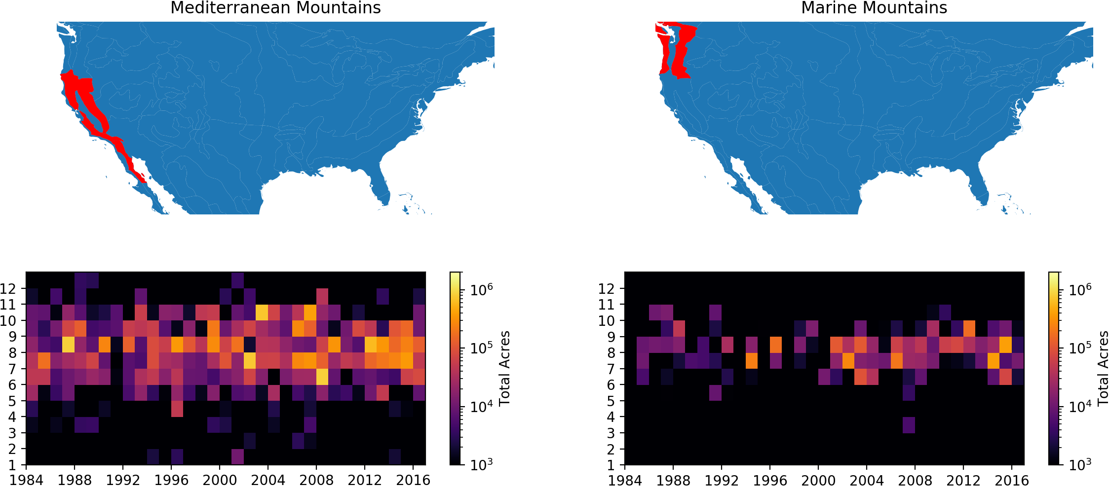
To do this, we started by creating a theoretical distribution of fire sizes across the 24 Bailey ecoregion divisions of the continental United States following methods developed by Bruce Malamud and others (see Figure 1).

Figure 1. Fitting theoretical curves to 23 years of fire events, by Bailey ecoregion division. The Y axis is frequency of events per km2 of land within the ecoregion; the X axis is the binned fire size.
Using a long-term database of wildfire events compiled by the USDA Forest Service, we applied Malamud’s approach to build cumulative probability distributions of fire size and frequency by ecosystem. This allows us to randomly sample the distribution for a given ecosystem, and the distribution will return a “fire event” with a predicted size. The shape of the logarithmic curves in Figure 1 tell us that smaller fires occur much more frequently than large fires, so each random sample is more likely to return a fire of modest size (a few acres in size or less), and only rarely will it return a massive fire (50,000 to 500,000+ acres, depending on the ecosystem). If we sample each distribution enough times, we can build a simulated “inventory” of fire events.
But, you might ask, how is an “inventory” of random samples from a statistical distribution representative of anything, let alone a “typical” year? Well, it isn’t, but here’s where it gets interesting. If we run our simulated inventory process over and over again, we start to re-create the inter-annual variability of fire events across ecosystems. Figure 2 below shows the results from 100 unique simulated inventories (100 virtual fire years), for both total area burned and the largest individual fire size (for a discussion of where 2020 falls within these predictions, see below). Now, we can pick an individual “year” for each ecoregion meeting the criteria we need for a given application. For the regional haze application, our “typical” inventory could be the simulation with the median total acres burned for each ecosystem. If instead we wanted to look at an extreme year, we could pick the 90th percentile total acres simulation. The key is, if we have a target of total acres burned, the simulation produces a distribution of fire sizes that (in general) conforms to recent historical activity across ecosystems.
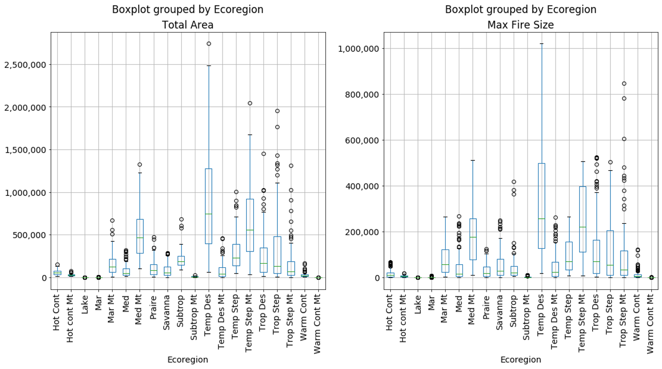
Figure 2. Results of running 100 virtual year simulations by ecosystem summarized by total area burned and largest individual fire event.
There is a long list of caveats, limitations, and nuances to this approach (not to mention how to actually distribute fires in space and time for a virtual year), and much more detail can be found in the final report that describes how the fire EIs for Round 2 of the Regional Haze process were developed. This approach was used to develop a 5-year representative baseline fire EI as well as a future-year scenario for the year 2028 that incorporated predictions of future biomass burning from ensemble climate modeling. To learn more about WRAP’s overall progress on Round 2 Regional Haze work, visit the Regional Haze Planning Work Group website.
This was a fun and challenging project to participate in, and we hope to find more uses for our “fire simulator” in the future.
A LOOK AT 2020
2020 was an unprecedented fire year both in California forests (“Med Mt” in the box plot figure) and the Pacific Northwest (“Mar Mt”). Based on how we constrained our model for the work described above, the maximum total acres predicted for California is 1.4MM acres, whereas the 2020 total was over 3.5MM. For the Pacific Northwest, the predicted max is 700K, but the 2020 total in Western Oregon alone exceeded 1MM.
In retrospect, we put too tight of bounds on our model by not letting the fitted curves go to a larger fire size bin beyond the largest reported fire in our historical dataset. We’re anxious to see what it would have predicted without these constraints. In addition, one of the cool things about the simulator framework is its ability to “learn”: as new historical fire activity is added, the probability distributions self-adjust, and the predicted outcomes will change.
We hope to have the opportunity for further applications of this work. If we do, we’ll be sure to share!
